Demographic Impact on Investment

Author

Collin Real

Published

July 26, 2024

SRI LAKSHMIR CHUNDRU contributed to this exercise.

1 Summary/Abstract

The analysis’s objective is to understand the insights and patterns recognized between customer demographics and their financial situation.

2 Introduction

2.1 General Background Information

Customer demographics, such as religion, gender, height, and weight were analyzed to identify which of these demographics had more significant influences on an individual’s investments.

2.2 Description of data and data source

The two variables I added to the data sheet are Religion and Investments. The Religion variable seeks to identify the spiritual beliefs, if any, of each individual. The Investments variable represents the total fair market value of an individual’s investment accounts.

2.3 Questions/Hypotheses to be addressed

Can individual’s be clustered into groups based on their demographics and the fair market value of their investment accounts? If so, how do we use these clusters to gain a competitive advantage?

3 Methods

We used R to import, clean, and run analysis on the data.

3.1 Data aquisition

Dummy data was used for this report.

3.2 Data import and cleaning

3.2.0.1 Import libraries.

library(readxl) #for loading Excel files
library(dplyr) #for data processing/cleaning

Attaching package: 'dplyr'
The following objects are masked from 'package:stats':

    filter, lag
The following objects are masked from 'package:base':

    intersect, setdiff, setequal, union
library(tidyr) #for data processing/cleaning
library(skimr) #for nice visualization of data 
library(here) #to set paths
3.2.0.2 Import Data

data_location <- here::here("starter-analysis-exercise","data","raw-data","exampledata2.xlsx")
rawdata <- readxl::read_excel(data_location)
print(rawdata)
# A tibble: 14 × 5
   Height Weight Gender Religion     Investments
   <chr>   <dbl> <chr>  <chr>              <dbl>
 1 180        80 M      Christianity       11000
 2 175        70 O      Agnostic            5000
 3 sixty      60 F      Islam               6500
 4 178        76 F      Judaism             9000
 5 192        90 NA     Atheist            12000
 6 6          55 F      Christianity        3000
 7 156        90 O      Buddhism            4200
 8 166       110 M      Hinduism            6600
 9 155        54 N      Atheist             1200
10 145      7000 M      Agnostic            8700
11 165        NA F      Islam              12400
12 133        45 F      Mormonism           2600
13 166        55 M      Mormonism           9900
14 154        50 M      Buddhism            7300

3.2.0.3 Check Data

codebook <- readxl::read_excel(data_location, sheet ="Codebook")
print(codebook)
# A tibble: 5 × 3
  `Variable Name` `Variable Definition`                 `Allowed Values`        
  <chr>           <chr>                                 <chr>                   
1 Height          height in centimeters                 numeric value >0 or NA  
2 Weight          weight in kilograms                   numeric value >0 or NA  
3 Gender          identified gender (male/female/other) M/F/O/NA                
4 Religion        spiritual beliefs                     Christianity, Islam, Ju…
5 Investments     fmv of investments in dollars         numeric value, or NA    

3.2.0.4 Descriptive Statistics

dplyr::glimpse(rawdata)
Rows: 14
Columns: 5
$ Height      <chr> "180", "175", "sixty", "178", "192", "6", "156", "166", "1…
$ Weight      <dbl> 80, 70, 60, 76, 90, 55, 90, 110, 54, 7000, NA, 45, 55, 50
$ Gender      <chr> "M", "O", "F", "F", "NA", "F", "O", "M", "N", "M", "F", "F…
$ Religion    <chr> "Christianity", "Agnostic", "Islam", "Judaism", "Atheist",…
$ Investments <dbl> 11000, 5000, 6500, 9000, 12000, 3000, 4200, 6600, 1200, 87…
summary(rawdata)
    Height              Weight          Gender            Religion        
 Length:14          Min.   :  45.0   Length:14          Length:14         
 Class :character   1st Qu.:  55.0   Class :character   Class :character  
 Mode  :character   Median :  70.0   Mode  :character   Mode  :character  
                    Mean   : 602.7                                        
                    3rd Qu.:  90.0                                        
                    Max.   :7000.0                                        
                    NA's   :1                                             
  Investments   
 Min.   : 1200  
 1st Qu.: 4400  
 Median : 6950  
 Mean   : 7100  
 3rd Qu.: 9675  
 Max.   :12400  
                
head(rawdata)
# A tibble: 6 × 5
  Height Weight Gender Religion     Investments
  <chr>   <dbl> <chr>  <chr>              <dbl>
1 180        80 M      Christianity       11000
2 175        70 O      Agnostic            5000
3 sixty      60 F      Islam               6500
4 178        76 F      Judaism             9000
5 192        90 NA     Atheist            12000
6 6          55 F      Christianity        3000
skimr::skim(rawdata)
Data summary
Name rawdata
Number of rows 14
Number of columns 5
_______________________
Column type frequency:
character 3
numeric 2
________________________
Group variables None

Variable type: character

skim_variable n_missing complete_rate min max empty n_unique whitespace
Height 0 1 1 5 0 13 0
Gender 0 1 1 2 0 5 0
Religion 0 1 5 12 0 8 0

Variable type: numeric

skim_variable n_missing complete_rate mean sd p0 p25 p50 p75 p100 hist
Weight 1 0.93 602.69 1922.25 45 55 70 90 7000 ▇▁▁▁▁
Investments 0 1.00 7100.00 3580.50 1200 4400 6950 9675 12400 ▇▅▇▇▇

3.2.0.5 Data Cleaning

d1 <- rawdata %>% dplyr::filter( Height != "sixty" ) %>% 
                  dplyr::mutate(Height = as.numeric(Height))

d2 <- d1 %>% dplyr::mutate( Height = replace(Height, Height=="6",round(6*30.48,0)))

d3 <- d2 %>%  dplyr::filter(Weight != 7000) %>% tidyr::drop_na()
d3$Gender <- as.factor(d3$Gender)
d4 <- d3 %>% dplyr::filter( !(Gender %in% c("NA","N")) ) %>% droplevels()  
processeddata <- d4
processeddata
# A tibble: 9 × 5
  Height Weight Gender Religion     Investments
   <dbl>  <dbl> <fct>  <chr>              <dbl>
1    180     80 M      Christianity       11000
2    175     70 O      Agnostic            5000
3    178     76 F      Judaism             9000
4    183     55 F      Christianity        3000
5    156     90 O      Buddhism            4200
6    166    110 M      Hinduism            6600
7    133     45 F      Mormonism           2600
8    166     55 M      Mormonism           9900
9    154     50 M      Buddhism            7300

3.3 Statistical analysis

One linear model was created with height as our dependent variable and weight/religion as our predictors.

4 Results

4.1 Exploratory/Descriptive analysis

?@tbl-summarytable shows a summary of the data.

Table 1: Data summary table.
skim_type skim_variable n_missing complete_rate factor.ordered factor.n_unique factor.top_counts numeric.mean numeric.sd numeric.p0 numeric.p25 numeric.p50 numeric.p75 numeric.p100 numeric.hist
factor Gender 0 1 FALSE 3 M: 4, F: 3, O: 2 NA NA NA NA NA NA NA NA
numeric Height 0 1 NA NA NA 165.66667 15.97655 133 156 166 178 183 ▂▁▃▃▇
numeric Weight 0 1 NA NA NA 70.11111 21.24526 45 55 70 80 110 ▇▂▃▂▂

4.2 Basic statistical analysis

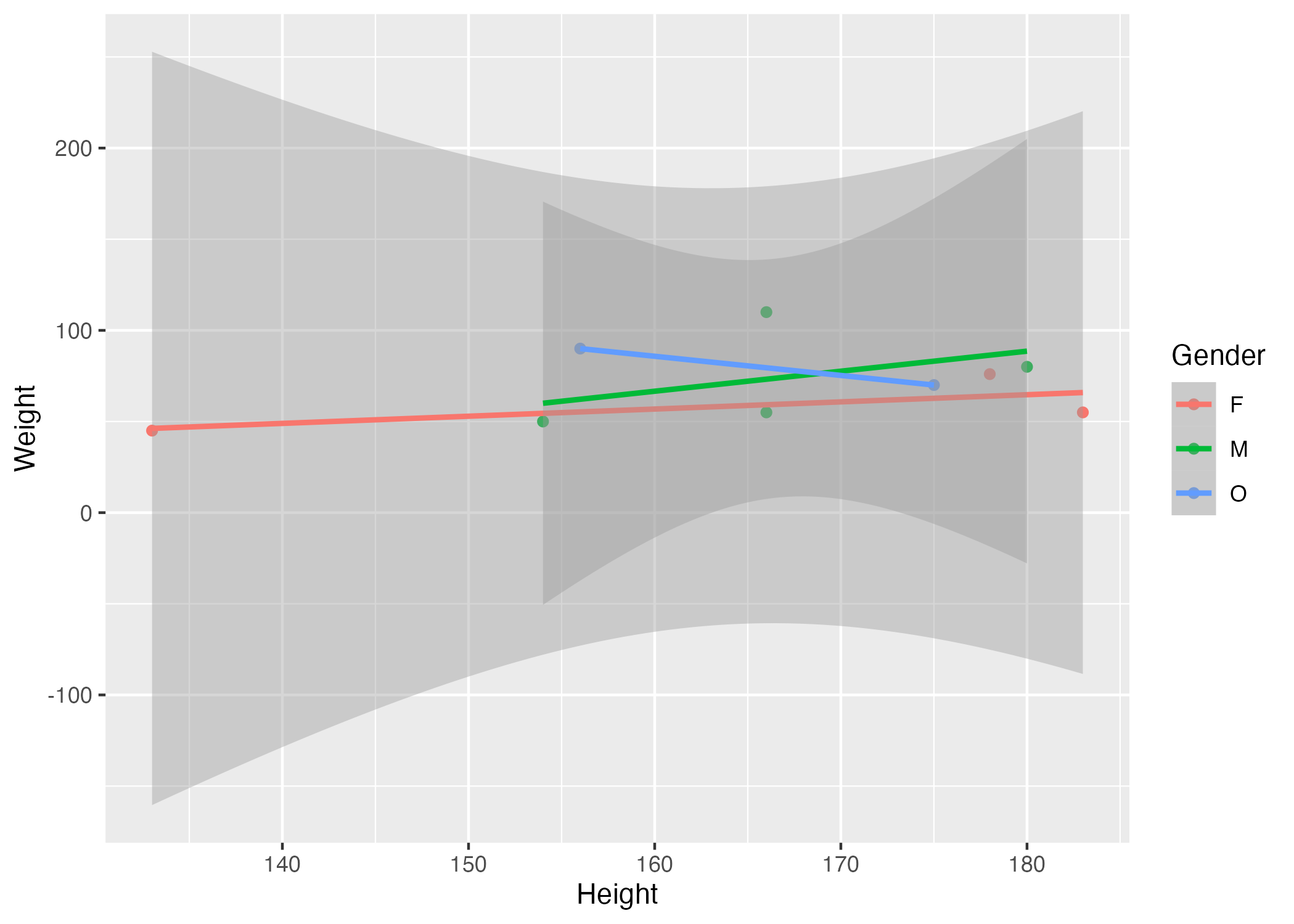
Figure 1 shows a scatterplot figure produced by one of the R scripts.

Figure 1: Height and weight stratified by gender.

4.3 Full analysis

Example Table 2 shows a summary of a linear model fit.

Table 2: Linear model fit table.
term estimate std.error statistic p.value
(Intercept) 149.2726967 23.3823360 6.3839942 0.0013962
Weight 0.2623972 0.3512436 0.7470519 0.4886517
GenderM -2.1244913 15.5488953 -0.1366329 0.8966520
GenderO -4.7644739 19.0114155 -0.2506112 0.8120871

4.3.1 Distribution of Height by Religion

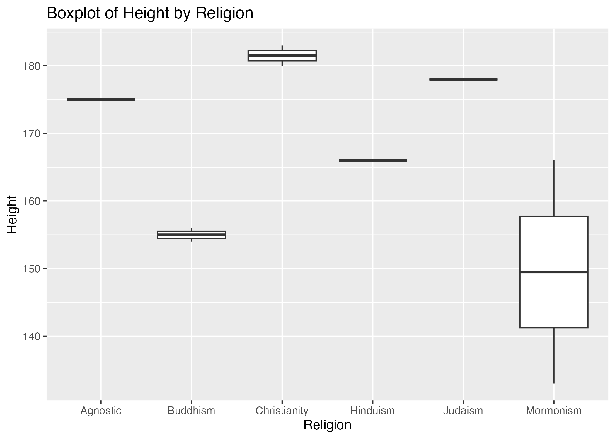
Figure 2: Distribution of height by religion.

4.3.2 Correlation Between Investments and Weight

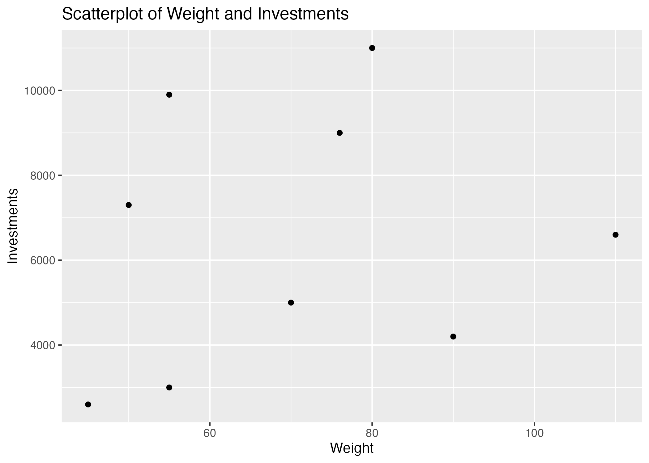
Figure 3: The relationship between investments and weight.

4.3.3 Investments/Religious Influence on Height

Table 3: Linear model fit table.
term estimate std.error statistic p.value
(Intercept) 164.913979 37.0650265 4.4493150 0.0469828
Weight 0.144086 0.4760345 0.3026798 0.7907129
ReligionBuddhism -20.000000 19.8783599 -1.0061192 0.4203016
ReligionChristianity 6.860215 19.9139524 0.3444929 0.7633274
ReligionHinduism -14.763441 29.8234767 -0.4950275 0.6696182
ReligionJudaism 2.135484 23.1305752 0.0923230 0.9348565
ReligionMormonism -22.618280 22.0407063 -1.0262048 0.4126949

5 Discussion

5.1 Summary and Interpretation

Two diagnostic plots were created to visualize the data. The box plot identifies the distribution of data among the categorical variable Religion and helps identify potential outliers. Our box plots demonstrate few variation in height for all religions except Mormonism. The scatter plot illustrates the relationship between the Weight and Investments variables (i.e. their degree of correlation). The scatter plot does not show much correlation between the two variables.

5.2 Strengths and Limitations

One major limitation is the small sample size. It’s difficult to identify patterns when a lack of data is present. Another limitation is not creating additional plots for other combinations of variables. One strength is the level of demographic data which is essential for market segmentation.

5.3 Conclusions

One of the key takeaways from this project is the importance of data acquisition and validating it’s integrity. Small samples sizes and junk data limit the opportunity of producing valuable insights. Data is the most critical asset for predictive modeling. If the integrity of a dataset is in question, so are the results of every model built on top of it.

This paper (Leek & Peng, 2015) discusses types of analyses.

These papers (McKay, Ebell, Billings, et al., 2020; McKay, Ebell, Dale, Shen, & Handel, 2020) are good examples of papers published using a fully reproducible setup similar to the one shown in this template.

Note that this cited reference will show up at the end of the document, the reference formatting is determined by the CSL file specified in the YAML header. Many more style files for almost any journal are available. You also specify the location of your bibtex reference file in the YAML. You can call your reference file anything you like, I just used the generic word references.bib but giving it a more descriptive name is probably better.

6 References

Leek, J. T., & Peng, R. D. (2015). Statistics. What is the question? Science (New York, N.Y.), 347(6228), 1314–1315. https://doi.org/10.1126/science.aaa6146
McKay, B., Ebell, M., Billings, W. Z., Dale, A. P., Shen, Y., & Handel, A. (2020). Associations Between Relative Viral Load at Diagnosis and Influenza A Symptoms and Recovery. Open Forum Infectious Diseases, 7(11), ofaa494. https://doi.org/10.1093/ofid/ofaa494
McKay, B., Ebell, M., Dale, A. P., Shen, Y., & Handel, A. (2020). Virulence-mediated infectiousness and activity trade-offs and their impact on transmission potential of influenza patients. Proceedings. Biological Sciences, 287(1927), 20200496. https://doi.org/10.1098/rspb.2020.0496